PostgreSQL & Grafana – Real-time data processing pipeline – Part 6

Believe it or not, we are getting to the end of this small series about a potential real-time data processing pipeline.
In this final part I will show how Grafana can retrieve our pipeline data from PostgreSQL and visualize it as a graph. But before we dive into it, let’s have a quick recap of the previous topics.

• Visual time series data generation
• OSC to ActiveMQ
• ActiveMQ, Spark & Bahir
• Data transformation
• Spark to PostgreSQL

So the bit that is still missing, is the visualization of data.

Starting the docker image

To keep things simple, I will use Grafana via the official docker image and start it up using the following command.

docker run -d --name=grafana -p 3000:3000 grafana/grafana 

For more information about the different configuration options, check out the link below.

https://grafana.com/docs/installation/docker/

Log In

As you can guess from the docker command above, the Grafana web UI is accessible via port 3000. Once connected, the following login screen is shown.

The default username and password are set to admin/admin and after logging in the first time, you are asked to change your password.

Define a PostgreSQL data source

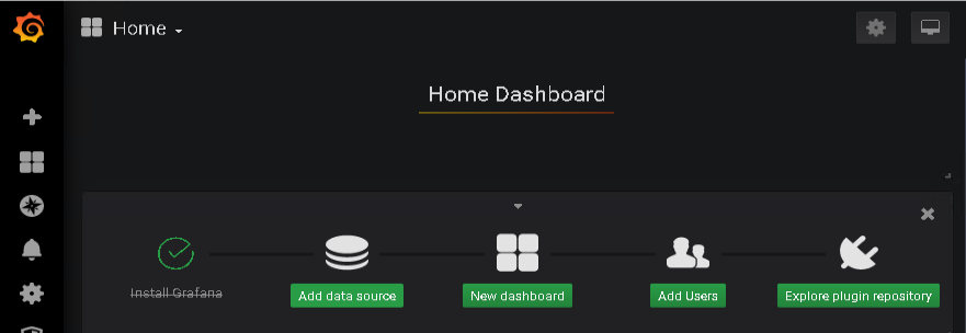
For PostgreSQL & Grafana to work together, I first have to define a data source. Therefore, I just select the “Add data source” option …

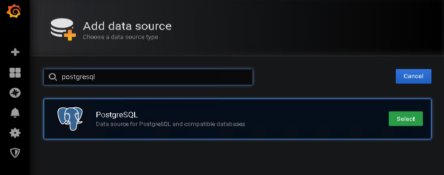
… and use the search field to look up PostgreSQL. Clicking the Select button takes me to the specific data source configuration settings.

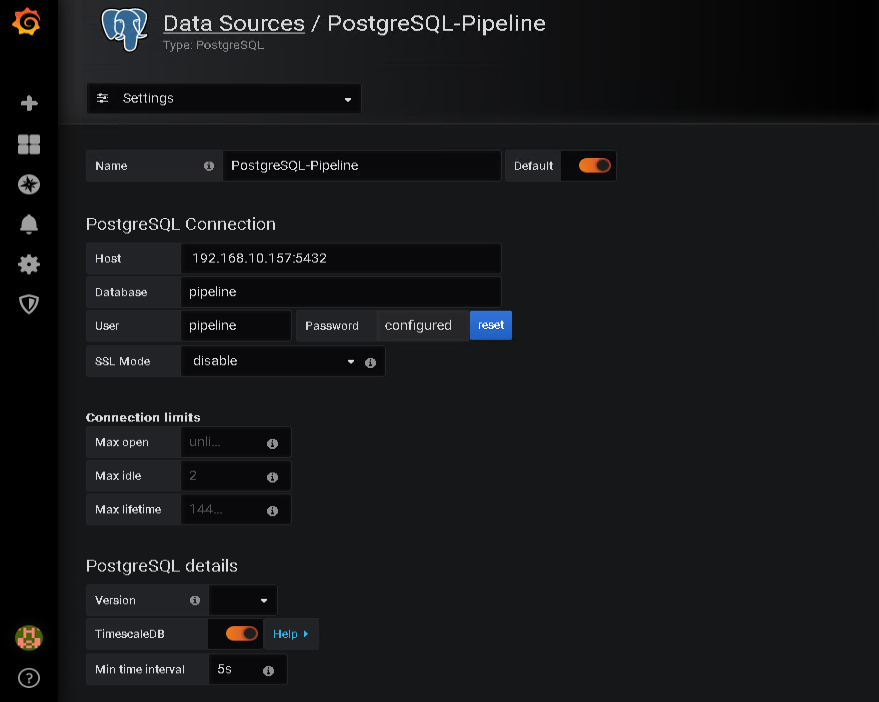
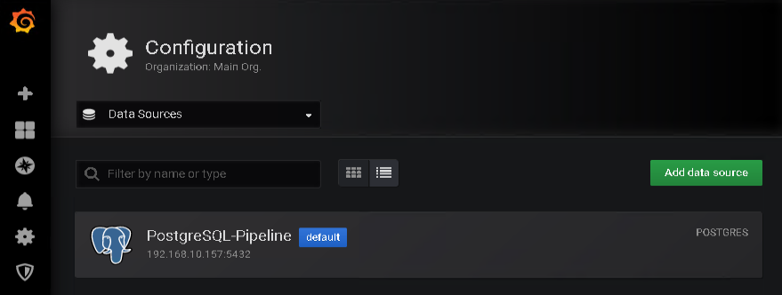
First, I need to provide a name for the data source. I’ve used “PostgreSQL-Pipeline” in the screenshot below.

Besides specifying the Host, Database and User, the other interesting configuration for me is the “TimescaleDB” option. As mentioned in the previous part of this series, I am using the TimescaleDB extension for testing and therefore enabled this option. If you do use plain PostgreSQL, just leave this off.

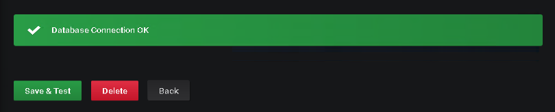
If everything is configured correctly, you should be able to connect to the database and get this confirmation message after pressing “Save & Test”…

… and the new Data Source should be visible as default source

Create the dashboard

Going back to the Grafana home page, I can now use the “New dashboard” option to navigate to the related configuration page and setup my first dashboard.

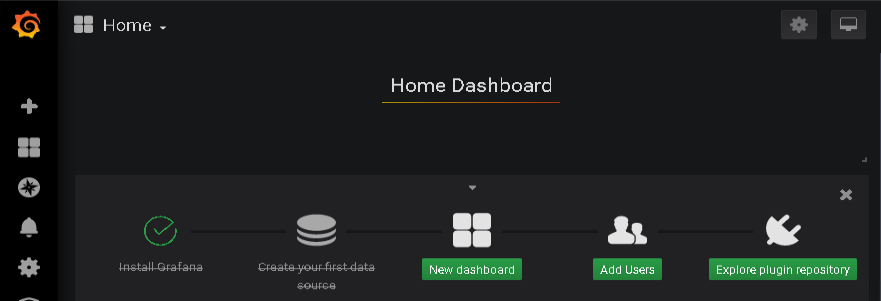
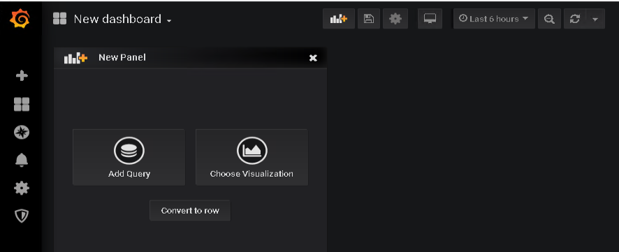
To define what data should be visualized, I choose “Add Query”, which takes me to the query editor.

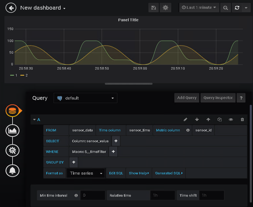
My data comes from the sensor_data table and therefore, this is what I use in the FROM field.

For the Time column field, I can use the sensor_time column of the sensor_data table. It defines the x-axis of the graph.

The Metric column defines the sensor that the data actually belongs to. As you probably can envision, in my case that is the sensor_id column.

SELECT is used for the data that is displayed on y-axis. In the sensor_data table, this is store in the column named sensor_value.

I now can save the dashboard …

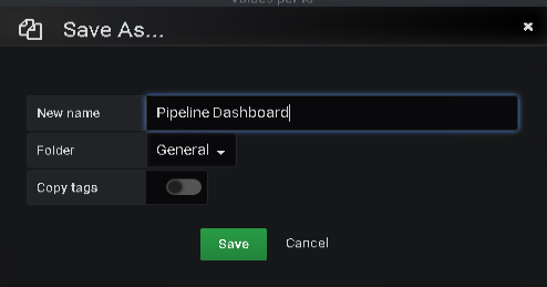
… and watch the data coming in.

Epilogue

That’s it. Yes, that was the final post of this mini series that outlined a potential real-time data processing pipeline. If you followed along, you now should be able to test out the different bits and pieces yourself.

I hope you enjoyed this mini series and, if you have any comments or questions, please feel free to get in touch via the contact form.

All the best and have a great time!