Real-time data processing pipeline – Part 1 – Visual time series data generation

This is the first part of my series to showcase a potential pipeline for real-time data processing. An overview about the different components that I am going to use can be found here.
So let’s get started and find out how real-time sensor data can be simulated, as each pipeline needs to start somewhere.

Introduction

There may be times when you need to generate continuous numeric data that allows you to test your real-time streaming processing pipeline. One common approach is to generate this data by code, which, however, can come with some drawbacks.

• A developer is required to generate the test data.
• The process engineer & developer need to work very closely together.
• A process change may require a change in code as well.
• Complex processing pipelines can lead to very complex code.
• Developing the generating code can take a lot of time.

Now consider an option that would allow a non-developer to draw and generate that test data in a visual tool in real-time. Doesn’t that sound useful?

Looking (a bit) out of the box

Believe it or not, I enjoy doing other things outside of the IT world as well. Producing electronic music is one of them, for example.

One of the most fun bits of producing electronic music is, to work with all sort of fancy controllers that are available nowadays. Like the Zoom ARQ shown below …

… or the Oddball, for example.

Most of these controllers use MIDI to send related messages to a connected instrument. MIDI has some limitations however, and that is one of the reasons why the Open Sound Control (OSC) protocol has been developed. It allows controlling more expressive instruments, but is also used to control robots for example.

I won’t go into the details of OSC, but some features, that make it useful for what I am trying to achieve, are:

• Data is transmitted over the network via UDP or TCP
• High-resolution timestamp (64-bit timetag) support
• Supports data-types like int32, float32 and string

Another really nice thing about OSC is the availability of OSC software out there.

Using IanniX for data generation

The description on the IanniX page states:

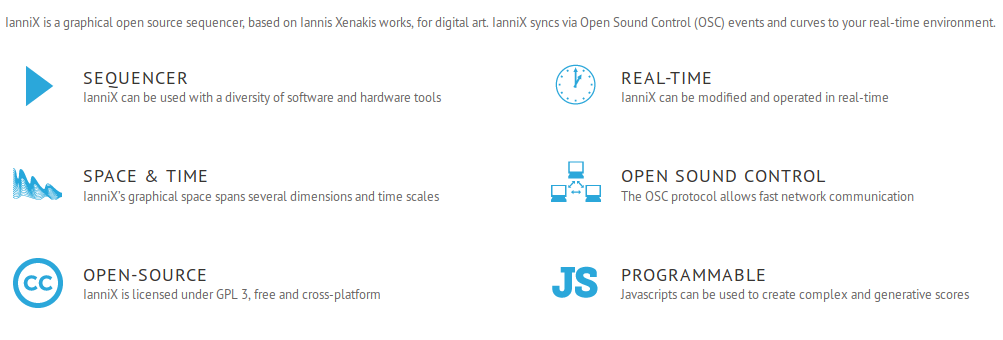
IanniX is a graphical open source sequencer, based on Iannis Xenakis works, for digital art. IanniX syncs via Open Sound Control (OSC) events and curves to your real-time environment.

“… event and curves … real-time …” Doesn’t that ring a bell?

Oh, and by the way, it’s open source and runs on OS X, Linux and Windows.

Simulating a temperature sensor

Now let’s build our first graph, simulating the data of a temperature sensor for example.

After you downloaded and started IanniX, you are presented with the initial screen. This is no in-depth IanniX tutorial, therefore I recommend that you also download the documentation and familiarize yourself with the basic functionality.

Create / Import your graph

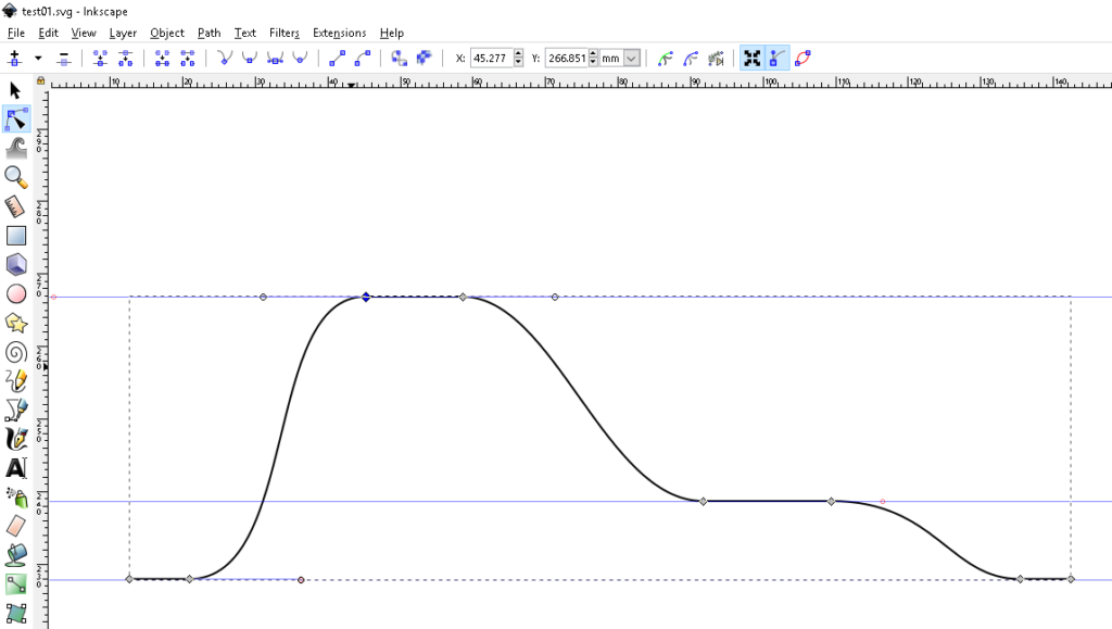
Of course, you can create your first graph directly in IanniX, but for more complex drawings (which this example isn’t), I find it much easier to create an SVG file via Inkscape, which then can be imported into IanniX.

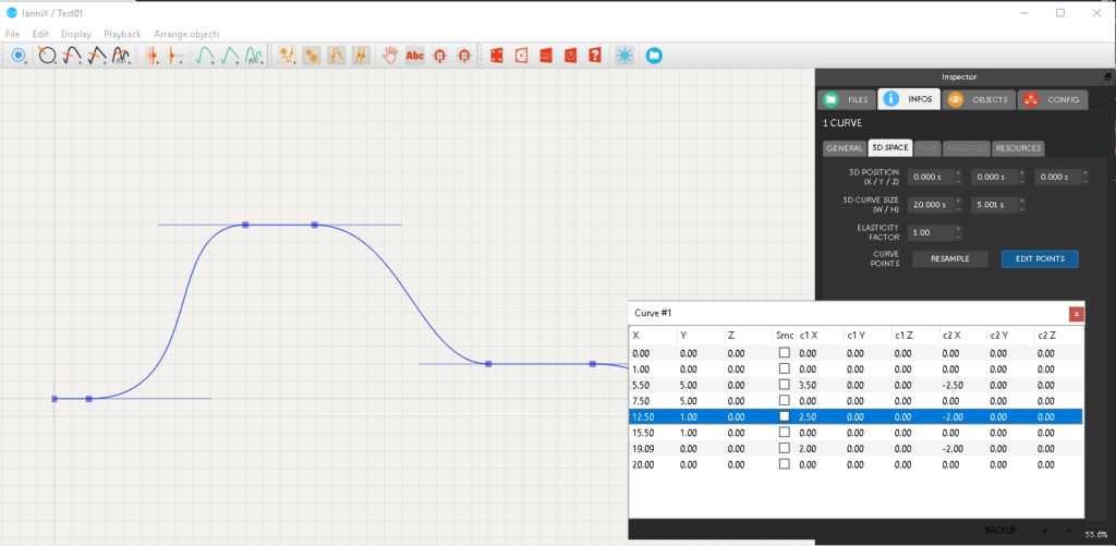
Once I imported the graph, I can further adjust any points via the UI, or use the “EDIT POINTS” button under the “INFOS” > “3D SPACE” section of the Inspector pane.

Add a cursor

Now add a cursor to your graph.

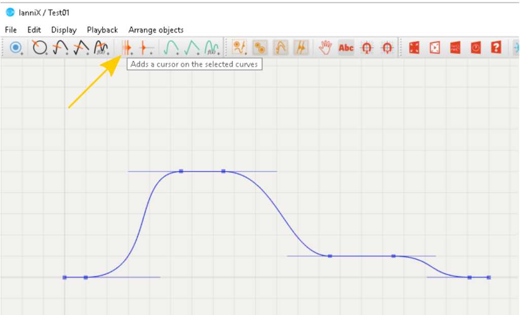
The location of the cursor helps to visualize what data will be transferred at a specific point in time. In our case, the X-axis represents the time and the Y-axis the temperature value.

Now, press the play-button, and you should see the cursor moving along the curve.

Adjust messages

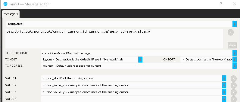
Next, select the cursor object and remove / adjust the messages that will be generated / sent. To do this, navigate to “INFO” > “MESSAGES” and click the “EDIT MESSAGE(S)” button.

Ensure that you have only one (OSC) message configured, similar to what is shown on the screenshot below.

Adjusting the generated values

The bounding box provides an indication about the min and max values that will be generated. Looking at the current box, you may notice two things.

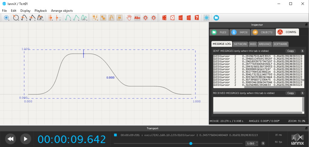
1. The values range from 0.000 to 1.000 for both axis, only.
2. It looks like the mix and max values are actually not reached. This can be confirmed by looking at the “MESSAGE LOG” window of the “CONFIG” tab.

I can resolve both issues via the options on the “INFOS” > “MESSAGES” tab.

By settings the mapping option to “Mapped on curves bounding rectangle” I will fit the bounding box to the graph, fixing the second issue.

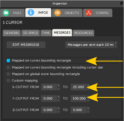
For my Y-axis, which is simulating the temperature, I want to generate values from 0 to 100. The X-axis values should range from 0 to 25, just to match the duration of the simulation. Adjusting the related OUTPUT values allows me to set the required ranges.

BTW: It is also possible to change the sample rate via the “Messages are sent each xx ms” option. The default is 20ms, which translates to 50 samples per second (50 Hz).

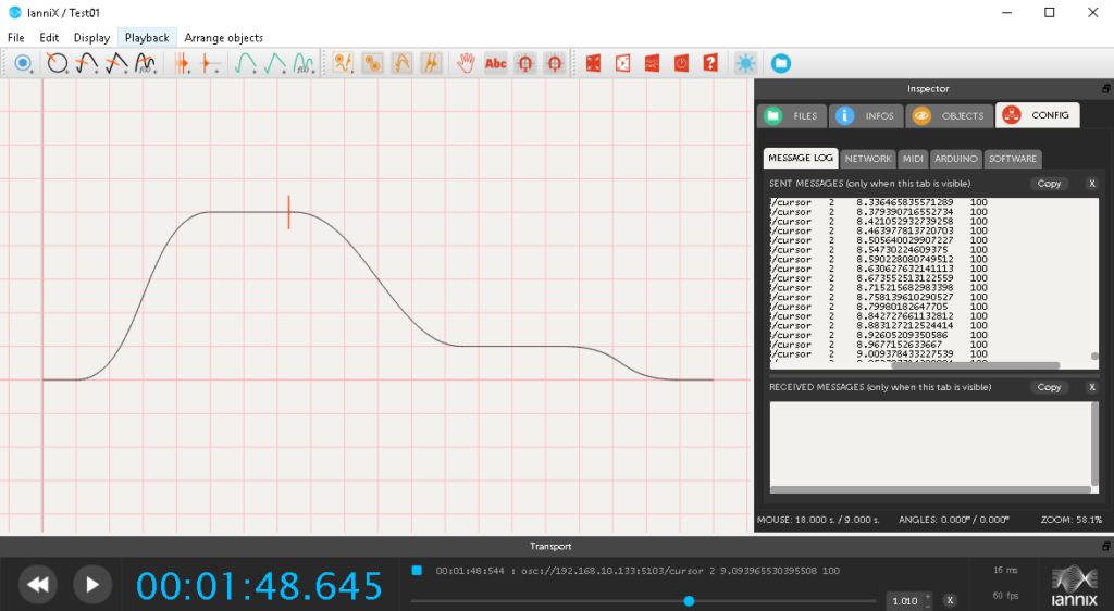
With the new settings in place, I now get the Y-values I want.

Fix timing

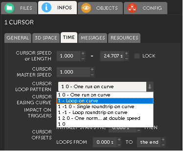
Finally, there are two additional settings, related to the cursor timing, that I want to modify.

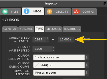
Per default the cursor runs only once, from start to the end. However, IanniX also supports different loop modes. For my purpose, “Loop on curve” is exactly what I need, as it just continues from the start, once the end has been reached.

As mentioned earlier, I want the full graph cycle to last 25 seconds. By specifying the cursor length, the cursor speed is automatically adjusted.

Now it’s time to view the final result.

Summary & Outlook

Hopefully this article about visual time series data generation in real-time sparked some ideas about how IanniX can be utilized for that purpose. Play around with it, add some more/other graphs and also explore how events can be simulated using triggers.

Obviously, generating the test data is just one part of the real-time processing story. In the next part of this series, I will build an example OSC receiver in C# and get IanniX connected to it.

So stay tuned and have a great time!