htm.core parameters – Single Order Sequence Memory

To allow the htm.core temporal memory to learn sequences effectively, it is import to understand the impact of the different parameters in more detail.

In this part I will introduce

• columnDimensions
• cellsPerColumn
• maxSegmentsPerCell
• maxSynapsesPerSegment
• initialPermanence
• connectedPermanence
• permanenceIncrement
• predictedSegmentDecrement

Temporal Memory – Previously on this blog…

Part 1 just covered enough basics of htm.core to get us started, and we actually saw how the single order memory got trained.
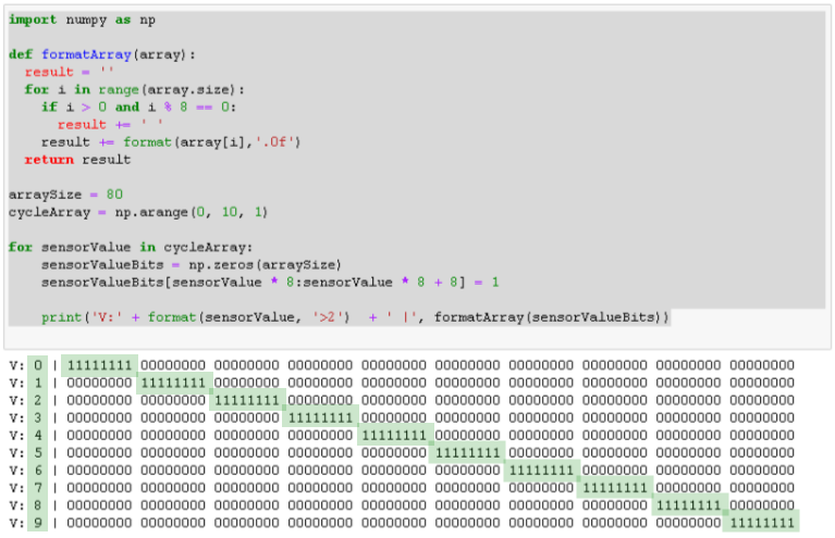
A cycle of encoded increasing numbers from 0 to 9 was very easy to predict, as there was always just one specific value that could follow the previous number.

Up and down

Now let’s see how the single order memory behaves, if things are not that obvious.
For that I will create a new range of encoded numbers that, after going from 0 to 9, will also go down to 0 again.

cycleArray = np.append( np.arange(0, 10, 1), np.arange(8, -1, -1))

Here is how that looks like, showing the number at the beginning of the line (V: x), followed by the encoded value. If you want, you can check part 1 for details about the encoding.

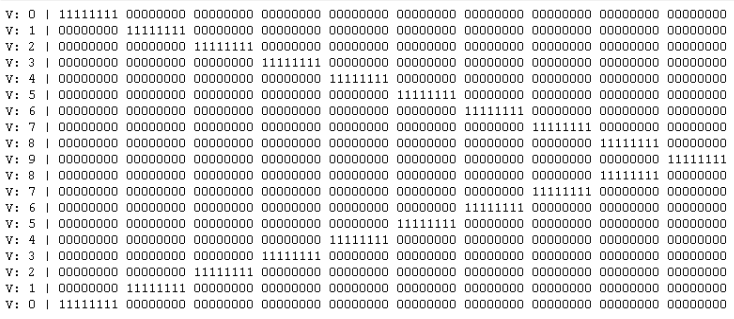
Showing the predicted values, we will see that, for the first time the Temporal Memory sees the descending values, it will just predict the same values that it has seen when the values were increasing.

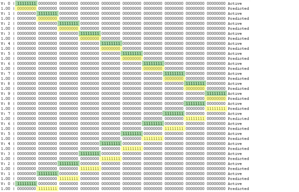
But what happens during the second cycle?

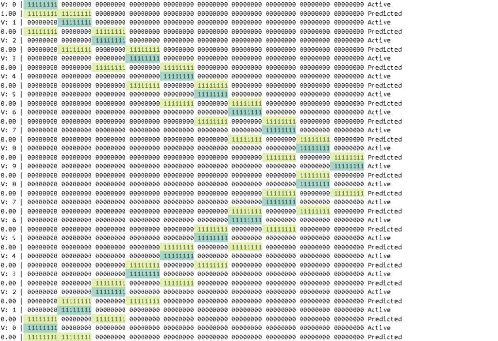
It actually detects the new pattern and remembers that for e.g. value 5 there can either follow value 4 or value 6. However, the Temporal Memory has no way of knowing which one is the correct value, yet.

Want to try this out yourself? Here’s the code:

import numpy as np
from htm.bindings.sdr import SDR
from htm.algorithms import TemporalMemory as TM

def formatSdr(sdr):
  result = ''
  for i in range(sdr.size):
    if i > 0 and i % 8 == 0:
      result += ' '
    result += str(sdr.dense.flatten()[i])
  return result

arraySize = 80
cycleArray = np.append( np.arange(0, 10, 1), np.arange(8, -1, -1))
inputSDR = SDR( arraySize )

tm = TM(columnDimensions = (inputSDR.size,),
        cellsPerColumn=1,       # default: 32
        minThreshold=1,         # default: 10
        activationThreshold=2,  # default: 13
        initialPermanence=0.5,  # default: 0.21
        )

for cycle in range(5):
    for sensorValue in cycleArray:
        sensorValueBits = inputSDR.dense
        sensorValueBits = np.zeros(arraySize)
        sensorValueBits[sensorValue * 8:sensorValue * 8 + 8] = 1
        inputSDR.dense = sensorValueBits

        tm.compute(inputSDR, learn = True)
        print('V:'+ format(sensorValue,'>2') + ' |', formatSdr(tm.getActiveCells()), 'Active')

        tm.activateDendrites(True)
        print(format(tm.anomaly, '.2f') + ' |', formatSdr(tm.getPredictiveCells()), 'Predicted')

But why is that the case and how can we change that?

To answer that, we need to understand a bit more about how the Temporal Memory is working and the meaning of the different parameters.

Temporal Memory – Simple console example

In the previous example, I have used an array of 80 bits to represent the numbers from 0 to 9.

This time, for simplicity’s sake, I am going to reduce this array to 8 bits and just encode the numbers 0 to 7, using one bit per number. I’ll also add a header to the output, showing the value and cycle along with the column index.

Therefore, the sequence of numbers for one cycle will now look like this:

cycleArray = [0, 1, 2, 3, 4, 5, 6, 7, 6, 5, 4, 3, 2, 1]

Please note, that the last number of the sequence is 1 and not 0.

Here is a preview of the output of the simple console application, with the active cell highlighted in green.

Don’t try this at home

To explore the different TM parameters, I’ll start with some settings that you probably won’t use in real-world scenarios, but this will help to understand their influence on the result.

columns = 8
inputSDR = SDR( columns )
cellsPerColumn = 1

tm = TM(columnDimensions          = (inputSDR.size,),
        cellsPerColumn            = cellsPerColumn,     # default: 32
        minThreshold              = 1,                  # default: 10
        activationThreshold       = 1,                  # default: 13
        initialPermanence         = 0.4,                # default: 0.21
        connectedPermanence       = 0.5,                # default: 0.5
        permanenceIncrement       = 0.1,                # default: 0.1
        permanenceDecrement       = 0.1,                # default: 0.1 
        predictedSegmentDecrement = 0.0,                # default: 0.0
        maxSegmentsPerCell        = 1,                  # default: 255
        maxSynapsesPerSegment     = 1                   # default: 255
        )

We will learn more about these parameters soon, but first…

A remark about terminology

Sometimes there may be confusion about the terms used in htm.core and how they map to the HTM theory. That’s where the following table might be able to assist.

htm.core	HTM theory
Column The htm.core default are 32 cells per mini-column (cellsPerColumn = 32)	Mini-Column (part of a Cortical Column)
Cell	Neuron (pyramidal)
Segment Each segment can have multiple connections htm.core default: maxSegmentsPerCell = 255	Distal dendritic segment
Connection – Connected—permanence is above the threshold. – Potential—permanence is below the threshold. – Unconnected—does not have the ability to connect. htm.core default: maxSynapsesPerSegment = 255	Synapse

More information about the terminology used in relation to the Temporal Memory is available via https://numenta.org/resources/HTM_CorticalLearningAlgorithms.pdf chapter 2, the HTM Cheat Sheet and https://numenta.com/assets/pdf/temporal-memory-algorithm/Temporal-Memory-Algorithm-Details.pdf.

Columns & Cells

columnDimensions & cellsPerColumn

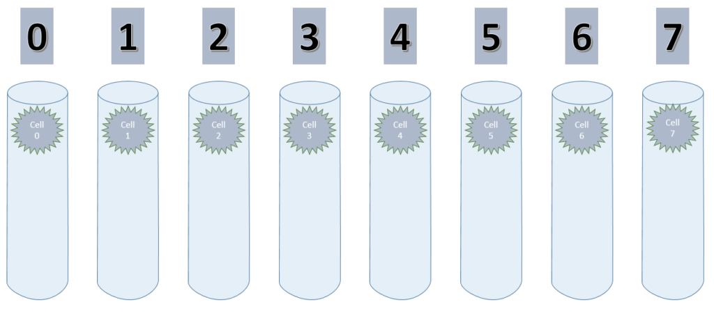
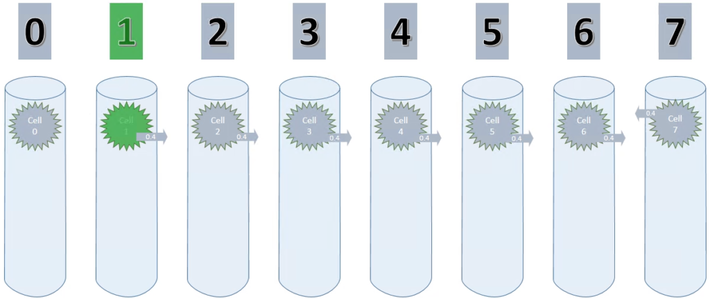
As explained earlier, there are 8 values to encode, using 1 bit per value. Each bit is handled by one column and therefore this is set to 8.

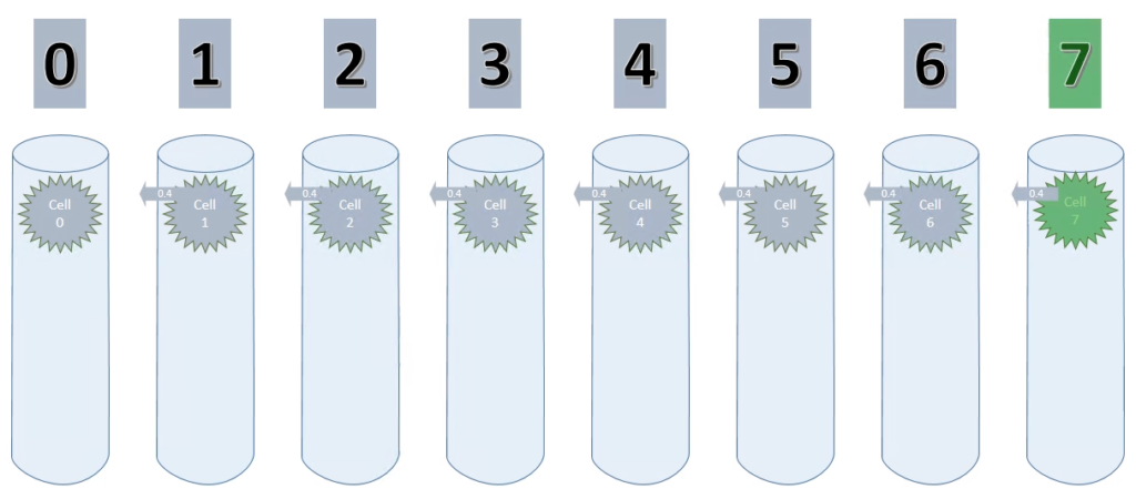
Considering that I only use one cell per column (cellsPerColumn = 1) initially, this setup could be visualized like shown below.

Connections

maxSegmentsPerCell & maxSynapsesPerSegment

The purpose of the Temporal Memory is to learn a sequence over time and it does this by growing segments/connections to other cells that were previously active. That’s why the TM is sometimes also called Sequence Memory.

Or in other words: In HTM, sequence memory is implemented by the Temporal Memory algorithm. (https://numenta.com/resources/biological-and-machine-intelligence/temporal-memory-algorithm/)

By setting maxSegmentsPerCell & maxSynapsesPerSegment to 1, a cell can only ever create one connection to one other cell, as shown in the animation below.
As long as the values increase, the potential connection is pointing to the cell on the left. On decreasing values however, this connection has to be replaced with a new connection.

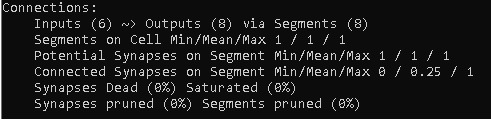
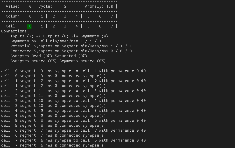
You can use the connection object, to print a useful connection summary as shown below.

print(tm.connections)

It is also possible to retrieve the actual connection details in htm.core. But be aware:

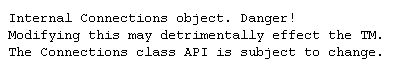
Anyway, the following code will print the connection details of a htm.core temporal memory.

def printConnectionDetails(tm):
    for cell in range(columns):
        segments = tm.connections.segmentsForCell(cell)

        for segment in segments:
            num_synapses = tm.connections.numSynapses(segment)
            for synapse in tm.connections.synapsesForSegment(segment):
                presynCell = tm.connections.presynapticCellForSynapse(synapse)                    
                permanence = tm.connections.permanenceForSynapse(synapse)
                print('cell', format(cell,'2d'), 'segment', format(segment,'2d'), 'has synapse to cell', format(presynCell,'2d'), 'with permanence', format(permanence,'.2f'))
            connected_synapses = tm.connections.numConnectedSynapses(segment)
            print('cell', format(cell,'2d'), 'segment', format(segment,'2d'), 'has', connected_synapses, 'connected synapse(s)')

So let’s use all of what we’ve learned so far to examine the first cycle of the console simulation.

Sequence Cycle 1

Cycle 1 – Step 1

Obviously, our fresh TM starts seeing the value 0, without any connections available yet.

What you can see however is, that we have 8 cells that are ready to establish connections: Outputs (8)

Cycle 1 – Step 2

This starts to get interesting, already. Now it has seen the new value (1) and started to create a connection.

The first line of the connections summary now shows Inputs (1), because one cell (cell 0) has a potential connection.

“Segments on Cell” tells us that there is at least one cell that does not have a segment (Min), at least one cell that does have a segment (Max) and also that 1/8 of all cells have a segment (Mean).

We also can see that we have one “Potential Synapses on Segment”, but no “Connected Synapses on Segment”, yet.

I’ll skip the last two summary lines for now, as they get more useful later.

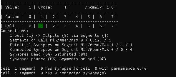
After the summary, detailed information about the connection from cell 1 is displayed.
In this case we see that cell 1 has 1 segment (with segment index 0), which in turn has a potential synapse to cell 0.

initialPermanence & connectedPermanence

It probably comes without any surprise that the permanence value of that synaptic connection is set to 0.40, as this is what we have set as the initialPermanence parameter for every new connection of a synapse.
To consider the synapse as connected, this value has to reach the value of the connectedPermanence value. 0.5 in this example.

Cycle 1 – Steps 3 to 8

The following steps up to step 8, in which the TM sees the value 7 the first time, don’t look much different.

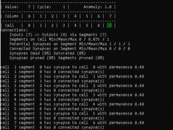
Looking back at the animation, this is where we are now.

Each cell (except cell 0) has a connection with a permanence of 0.4 to its sequence predecessor.

We can also see in the summary, that 7 cells (0 to 6) are receiving a connection now: Inputs (7)

Cycle 1 – Step 9

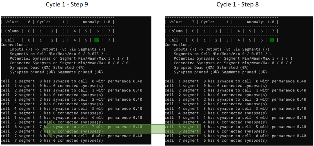
In step 9, the TM sees the value 6 the second time, but with the cell 7 as previously active cell. Therefore, it also wants to establish a connection from cell 6 to 7. However, as we have set maxSegmentsPerCell to 1, it has no other choice than to replace the old segment (index 5) with a new one (index 7).

Cycle 1 – Step 10 to 14

The behavior above is repeated for the remaining steps of the cycle, which leaves us with the following at step 14.

It might be worth noting, that the connection summary just displays 6 inputs. That is because we have 7 connections, but there are actually no incoming connections to cell 0 and 1.

Sequence Cycle 2

Cycle 2 – Step 1

The only thing special about this step is, that finally cell 0 has created a connection towards cell 1, resulting in 7 inputs in the connection summary.

Cycle 2 – Step 2 to 7

All the cells that get active in these steps need to establish new connections to the previously active cell again. That means that they actually do not have a chance to ever get beyond the connectedPermanence threshold of 0.5.

Cycle 2 – Step 8

That step actually is different. As – in this sequence – the previously active cell for cell 7 is always going to be cell 6, the TM does not need to create a new segment, but instead can increase the permanence value now.

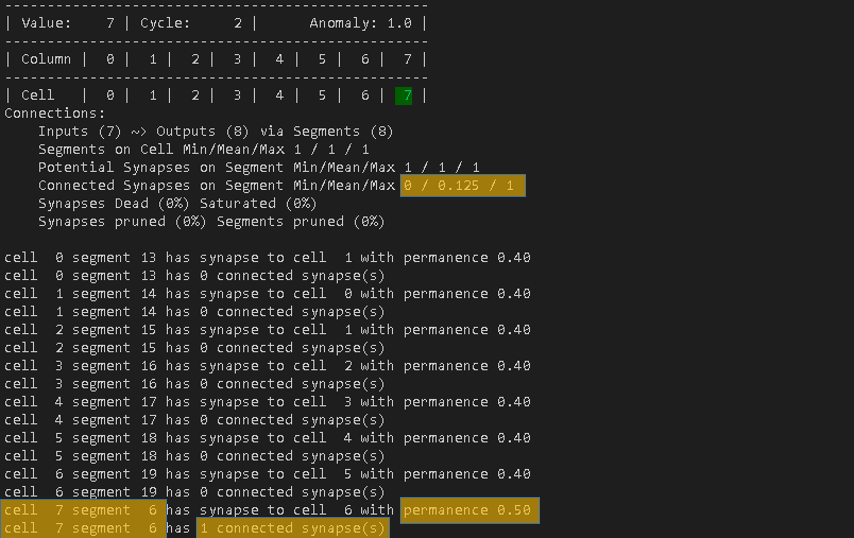
permanenceIncrement

For this test, the permanceIncrement is set to 0.1. By recalling the connectedPermanence of 0.5 and the initialPermanence of 0.4, the update to the connection from cell 7 now makes sense.

By seeing the connection again, it increased the previous permanence of 0.4 by 0.1. The new permanence is now set to 0.5 and therefore the synapse is considered as connected.

Cycle 2 – Step 9 to 14

In essence, these steps are similar to their corresponding step numbers in cycle 1. And again, because maxSegmentsPerCell is set to 1, all existing connections of these cells are replaced by new connections. Learning is just not possible.

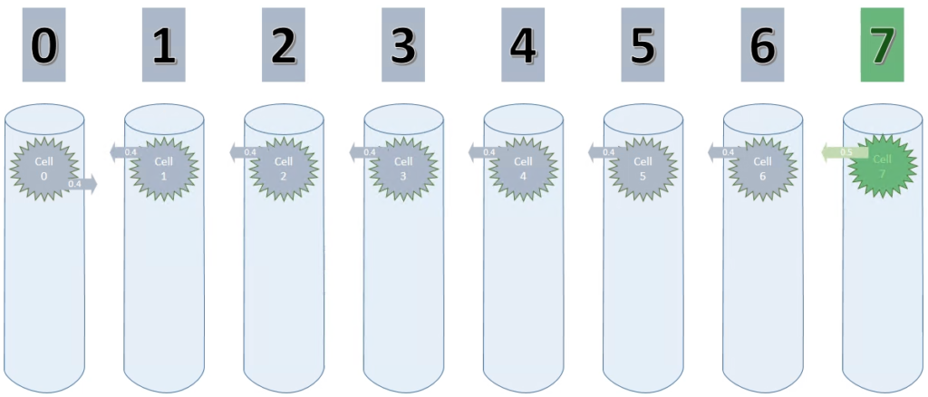
Cycle 3

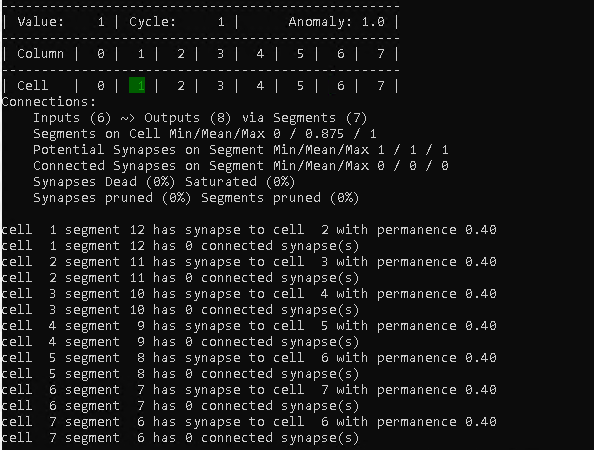
Below is the animation for cycle 3. Cell 0 is now connected to cell 1.

And here is a screenshot of the last step of cycle 3.

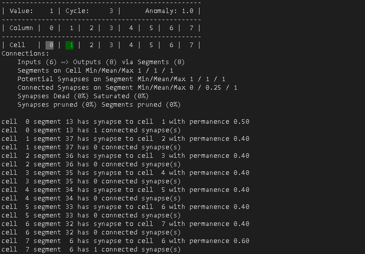
By the way. The cell in gray is the one that the TM predicts as next cell. This is because cell 0 has a connected synapse to cell 1, which is considers as connected.
Since the sequence is descending, the prediction is actually correct at the current step.

However, it will use the same prediction on the ascending sequence as well, which obviously is wrong.

It might be interesting to see what happens if I set the predictedSegmentDecrement to something else than 0. We’ll have a look at that soon, but for now, let’s just watch the temporal memory in action with the current settings.

Did you notice how the permanence of cell 0 and cell 1 continues to grow. If I add more cycles, they will do this until a permanence of 1 is reached.

Wrong prediction?

predictedSegmentDecrement

Earlier I’ve mentioned that some predictions of the temporal memory just cannot be correct in this example. This is where the predictedSegmentDecrement comes into the picture. Here is the definition as per htm.core.

Amount by which segments are punished for incorrect predictions.
          A good value is just a bit larger than (the column-level sparsity *
          permanenceIncrement). So, if column-level sparsity is 2% and
          permanenceIncrement is 0.01, this parameter should be something like 4% *
          0.01 = 0.0004

For my next example I just use a value of 0.05 to make things more obvious. So let’s have a look how this impacts the temporal memory.

Looking at cycle 1, step 10 and cycle 2, step 3 for example, you’ll notice that punishing already starts, even though no synapses are considered as connected yet. Decreasing the permanence to 0.35.

At cycle 2, step 8 the connection of cell 7 to cell 6 is increased again by the permanenceIncrement value and then punished again at step 10.
The same happens to the connection of cell 0 to cell 1 in step 1 and 3 of cycle 3.

As the permanenceIncrement is larger than the penalty of the predictedSegmentDecrement, cell 0 and 7 get connected eventually in this example. Nevertheless, I think you get the idea of why the predictedSegmentDecrement parameter might be useful.

Temporal Memory – Outlook

That’s it for this post and I hope you have a better understanding now, of why the temporal memory isn’t able to remember this simple sequence, yet.
In the next HTM related post, I’ll explore what settings need to be changes, so that it actually can and will successfully learn.

Oh… almost forgot. Here’s the example code in case you want to play around with it yourself.

import numpy as np
from htm.bindings.sdr import SDR
from htm.algorithms import TemporalMemory as TM
from time import sleep
from console import fg, bg, utils

def formatCell(cellName, activeState, winnerState, predictedState):
    styleFg = fg.white
    styleBg = bg.black
    style = None

    if(activeState == 1):
        styleFg = fg.green

    if(winnerState == 1):
        styleBg = bg.i22

    if(predictedState == 1):
        styleBg = bg.i241
    
    style = styleFg + styleBg
    if(style != None):
        result = style(format(cellName,'2d'))
    else:
        result = format(cellName,'2d')
    return result

def printHeader(step, sensorValue):
    print('-' * dashMultiplyer)
    print('| Cycle', format(cycle+1,'2d'), '| Step', format(step,'3d'), '| Value', format(sensorValue,'3d'),  '| Anomaly:', format(tm.anomaly, '.1f'), '|')
    print('-' * dashMultiplyer)

    colHeader = '| Column | '
    for colIdx in range(columns):
        colHeader +=  format(colIdx,'2d') + ' | '

    print(colHeader)
    print('-' * dashMultiplyer)

def printConnectionDetails(tm):
    for cell in range(columns * cellsPerColumn):
        segments = tm.connections.segmentsForCell(cell)

        for segment in segments:
            num_synapses = tm.connections.numSynapses(segment)
            for synapse in tm.connections.synapsesForSegment(segment):
                presynCell = tm.connections.presynapticCellForSynapse(synapse)                    
                permanence = tm.connections.permanenceForSynapse(synapse)
                print('cell', format(cell,'2d'), 'segment', format(segment,'2d'), 'has synapse to cell', format(presynCell,'2d'), 'with permanence', format(permanence,'.2f'))
            connected_synapses = tm.connections.numConnectedSynapses(segment)
            print('cell', format(cell,'2d'), 'segment', format(segment,'2d'), 'has', connected_synapses, 'connected synapse(s)')

def process(cycleArray):
    step = 1
    for sensorValue in cycleArray:
        sensorValueBits = inputSDR.dense
        sensorValueBits = np.zeros(columns)
        sensorValueBits[sensorValue] = 1
        inputSDR.dense = sensorValueBits

        tm.compute(inputSDR, learn = True)
        activeCells = tm.getActiveCells()
        tm.activateDendrites(True)

        activeCellsDense = activeCells.dense
        winnerCellsDense = tm.getWinnerCells().dense
        predictedCellsDense = tm.getPredictiveCells().dense

        utils.cls()
        printHeader(step, sensorValue)

        for rowIdx in range(cellsPerColumn):
            rowData = activeCellsDense[:,rowIdx]
            rowStr = '| Cell   | '
            for colI in range(rowData.size):
                cellName = np.ravel_multi_index([colI, rowIdx], (columns, cellsPerColumn))
                stateActive = activeCellsDense[colI,rowIdx]
                stateWinner = winnerCellsDense[colI,rowIdx]
                statePredicted = predictedCellsDense[colI,rowIdx]
                rowStr += formatCell(cellName, stateActive, stateWinner, statePredicted) + ' | ' 
            print(rowStr)
                
        print(tm.connections)
        printConnectionDetails(tm)
        print()
        step = step + 1
        sleep(0.5)

dashMultiplyer = 50

cycleArray = [0, 1, 2, 3, 4, 5, 6, 7, 6, 5, 4, 3, 2, 1]
cycles = 4

columns = 8
inputSDR = SDR( columns )
cellsPerColumn = 1

tm = TM(columnDimensions          = (inputSDR.size,),
        cellsPerColumn            = cellsPerColumn,     # default: 32
        minThreshold              = 1,                  # default: 10
        activationThreshold       = 1,                  # default: 13
        initialPermanence         = 0.4,                # default: 0.21
        connectedPermanence       = 0.5,                # default: 0.5
        permanenceIncrement       = 0.1,                # default: 0.1
        permanenceDecrement       = 0.1,                # default: 0.1 
        predictedSegmentDecrement = 0.0,                # default: 0.0
        maxSegmentsPerCell        = 1,                  # default: 255
        maxSynapsesPerSegment     = 1                   # default: 255
        )

for cycle in range(cycles):
    process(cycleArray)