Hierarchical Temporal Memory – part 1 – getting started

Prologue

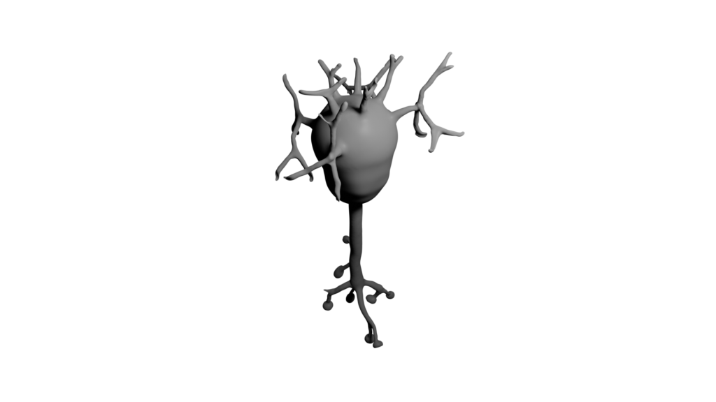
I came across the concept of Hierarchical Temporal Memory (HTM) and its implementation a while ago, and am still very fascinated about this approach to artificial intelligence.

When, about one year ago, the active development shifted towards the community fork named htm.core, which supports Python 3, it became finally time to have a closer look and try it out by myself.

BTW: According to this forum post, there are no plans to upgrade the older NuPIC library to Python 3.

A lot of documentation about the theory of HTM is available at numenta.org, already. Like this introduction to Biological and Machine Intelligence (BAMI) for example. There is also a great video tutorial series available on YouTube named HTM School. This probably might be the best starting point, if you are coming from a more technical background.

htm.core is developed in C++ and also provides bindings to Python 3 (which I will use). Bindings for C# are currently under development, and I am really looking forward to giving them a try, once they are available.

In some of my previous posts, like the series about a real-time data processing pipeline for example, I have used some generated time series sensor data for testing. As you will learn, HTM is an excellent candidate to be used for anomaly detection based on this kind of data.

When immersing yourself in HTM, you will discover many parameters to optimize the algorithm. However, I will try to reduce them to a very small subset in this post.

The core components of HTM

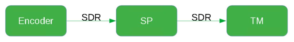
If you look into the examples that come with htm.core, you will notice that there are basically 4 main components that are used in a HTM application (like in the included hotgym.py example).

• Sparse Distributed Representation (SDR)
• Encoders
• Spatial Pooler (SP)
• Temporal Memory (TM)

Sparse Distributed Representation

As a developer who wants to get started with htm.core, let’s think of an SDR as just an object that is used to exchange information between the three other key components.

In fact, there is an SDR class that can be imported as shown below.

 from htm.bindings.sdr import SDR 

Obviously there is much more to it and I would like to refer you to the HTM School videos to have a closer look:

Encoders

Encoders are responsible for translating the input data into a format that HTM can work with. As we know already, in HTM terms, this target format is called SDR.

By the way: the encoded SDR – even though it is called Sparse Distributed Representation – doesn’t necessarily have to be sparse (more on that later)

Obviously there is also more to learn about encoders, and htm.core ships with a useful set, already (python -m pydoc htm.encoders) . However, for this getting started tutorial, I will just create a very minimalistic encoder.

Of course, if you want to dig into more details already, this paper about Encoding Data for HTM Systems by Scott Purdy, might be a good starting pace.

Spatial Pooler

A Spatial Pooler exists to achieve two main things:

• Turn a none-sparse representation into sparse representation, as the SDR created by an encoder doesn’t necessarily have to be sparse (see above)
• Detect overlapping input bits to enable grouping by semantic meaning

The Spatial Pooler is a complex topic by itself. But the good news is, that it is possible to use the temporal memory without it. Therefore, to keep things as simple as possible initially, I will skip the usage of a Spatial Pooler for now and come back to it in one of the future posts.

Temporal Memory

Learning and predicting is the domain of the temporal memory. As usual, HTM School has got this covered in much detail, already.

Using htm.core you can access the Temporal Memory using the following import

 from htm.algorithms import TemporalMemory as TM 

Coding Time

So let’s get started and build our very first htm.code application in python 3.
Focusing on the very basics in this post, I am going to

1. Create a semantic representation of the integer numbers from 0 to 9
2. Turn this representation into an SDR
3. Create a temporal memory and train it with the SDR
4. Have a look at the predictions of the TM after training

If you want to follow along and experiment with the code yourself, the htm.core-jupyter docker image, which is available at https://hub.docker.com/r/3rdman/htm.core-jupyter, might come in handy.

Creating the input sequence

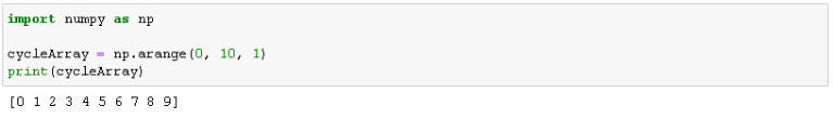
The first step is to create the input sequence. As you can see below, I am using NumPy to create a sequence of numbers from 0 to 9.

import numpy as np

cycleArray = np.arange(0, 10, 1)
print(cycleArray)

Bit representation

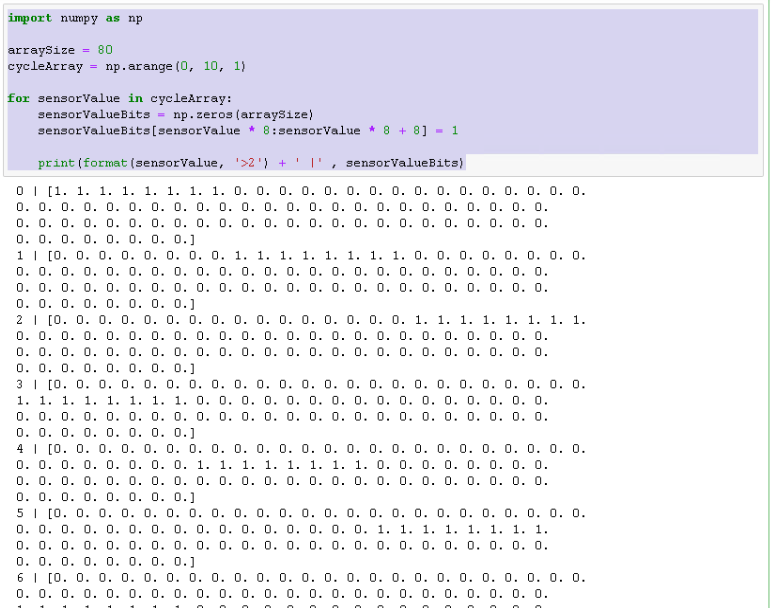
By now you probably know that you need to encode each kind of input into a bit-representation that htm.core can understand. Therefore, we need to convert each individual number in our sequence into an array of zeroes (inactive bits) and ones (active bits).

Another thing to be aware of is, that the Temporal Memory actually needs at list 8 active bits, to work as expected.

Keeping in mind that we have 10 numbers (0 to 9) and we need at least 8 active bits to represent every number, I set the array size to 80. We then can iterate over these numbers and set the active bits as shown below.

import numpy as np

arraySize = 80
cycleArray = np.arange(0, 10, 1)

for sensorValue in cycleArray:
    sensorValueBits = np.zeros(arraySize)
    sensorValueBits[sensorValue * 8 : sensorValue * 8 + 8] = 1

    print(format(sensorValue, '>2') + ' |' , sensorValueBits)

Beautify

The result looks a bit ugly. So let’s try to fix that by creating a python function named formatArray, that turns our bit-array into something more readable.

import numpy as np

def formatArray(array):
  result = ''
  for i in range(array.size):
    if i > 0 and i % 8 == 0:
      result += ' '
    result += format(array[i],'.0f')
  return result

arraySize = 80
cycleArray = np.arange(0, 10, 1)

for sensorValue in cycleArray:
    sensorValueBits = np.zeros(arraySize)
    sensorValueBits[sensorValue * 8 : sensorValue * 8 + 8] = 1
 
    print('V:' + format(sensorValue, '>2')  + ' |', formatArray(sensorValueBits))

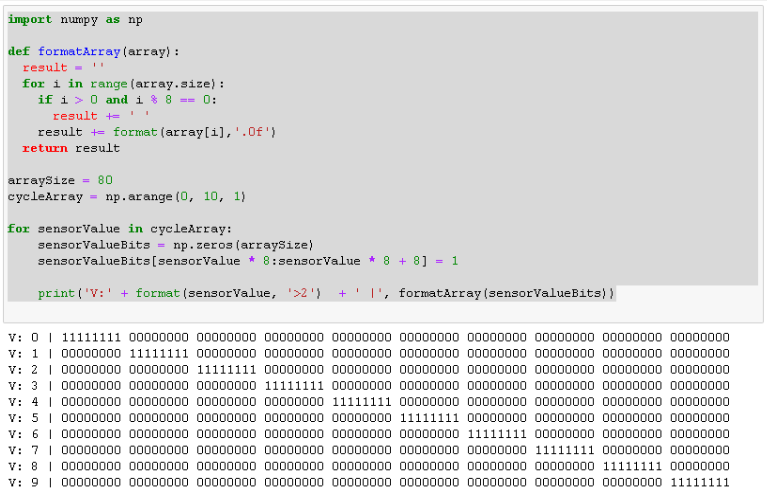
Much nicer to read, isn’t it?

Array to Sparse Distributed Representation

Before I turn the byte array into an SDR, it might be useful to have a quick look at the related documentation. Use the following command to display it in either the interactive python shell, or in Jupyter.

import htm.bindings.sdr
help(htm.bindings.sdr.SDR)

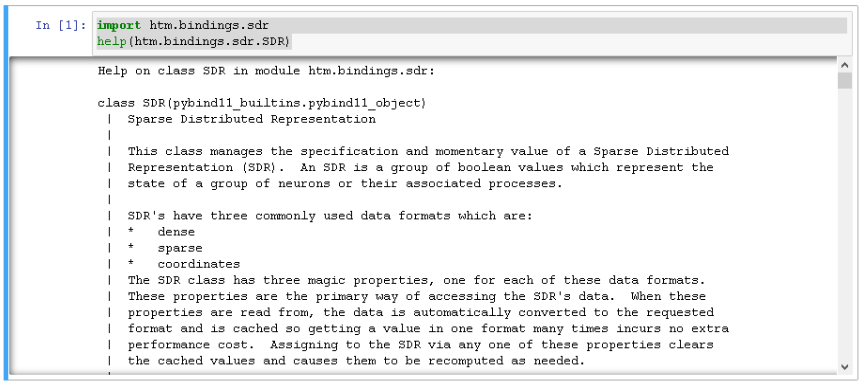
Reading through it, you might notice the following:

Assigning a value to the SDR requires copying the data from Python into C++. To avoid this copy operation: modify sdr.dense inplace, and assign it to itself.
This class will detect that it’s being given it’s own data and will omit the copy operation.

Example Usage of In-Place Assignment:
X = SDR((1000, 1000)) # Initial value is all zeros
data = X.dense
data[ 0, 4] = 1
data[444, 444] = 1
X.dense = data
X.sparse -> [ 4, 444444 ]

That’s useful information.
So lets first create our SDR object (line 14) with the same size as our array and then assign our encoded bits the recommended way (line 17 and 20).

import numpy as np
from htm.bindings.sdr import SDR

def formatArray(array):
  result = ''
  for i in range(array.size):
    if i > 0 and i % 8 == 0:
      result += ' '
    result += format(array[i],'.0f')
  return result

arraySize = 80
cycleArray = np.arange(0, 10, 1)
inputSDR = SDR( arraySize )

for sensorValue in cycleArray:
    sensorValueBits = inputSDR.dense
    sensorValueBits = np.zeros(arraySize)
    sensorValueBits[sensorValue * 8:sensorValue * 8 + 8] = 1
    inputSDR.dense = sensorValueBits

    print(sensorValue, ':', formatArray(sensorValueBits))

If you run this, you actually won’t notice any difference in the output. But, unless you get any errors, the assignment to the SDR was successful.

Adding the Temporal Memory

Almost there.
Now I can add the Temporal Memory and get it to learn our sequence.

I am initializing the TemporalMemory with the following code, leaving most of its default parameters untouched. I will try to explain the parameters in more detail in the future, but obviously you can get some additional insight from the documentation as well via help(htm.bindings.algorithms.TemporalMemory

tm = TM(columnDimensions = (inputSDR.size,),
        cellsPerColumn = 1,       # default: 32
        minThreshold = 4,         # default: 10
        activationThreshold = 8,  # default: 13
        initialPermanence = 0.5,  # default: 0.21
        )

Here is the full list of the parameters with their data type and default values, just in case you are curious.

• cellsPerColumn: int = 32
• activationThreshold: int = 13
• initialPermanence: float = 0.21
• connectedPermanence: float = 0.5
• minThreshold: int = 10
• maxNewSynapseCount: int = 20
• permanenceIncrement: float = 0.1
• permanenceDecrement: float = 0.1
• predictedSegmentDecrement: float = 0.0
• seed: int = 42
• maxSegmentsPerCell: int = 255
• maxSynapsesPerSegment: int = 255
• checkInputs: bool = True
• externalPredictiveInputs: int = 0
• anomalyMode: htm.bindings.algorithms.ANMode = ANMode.RAW

However, there is one “unusual” setting I have used, that deserves a bit more explanation.

cellsPerColumn = 1

By using just one cell per column, I basically enforce the Temporal Memory to work as single order memory only. Again, I am doing this to keep things as simple as a can for now. To learn more about single order memory vs. high order memory, watch the HTM School video below.

Learning

With the Temporal Memory initialized, we can actually tell it to learn each step of our sequence. This is done via tm.compute at line 30 of the code below.

To get the algorithm’s prediction, tm.activateDendrites needs to be called first (line 33).

Line 31 and 34 basically just print the actual SDR and then the prediction.

import numpy as np
from htm.bindings.sdr import SDR
from htm.algorithms import TemporalMemory as TM

def formatSdr(sdr):
  result = ''
  for i in range(sdr.size):
    if i > 0 and i % 8 == 0:
      result += ' '
    result += str(sdr.dense.flatten()[i])
  return result

arraySize = 80
cycleArray = np.arange(0, 10, 1)
inputSDR = SDR( arraySize )

tm = TM(columnDimensions = (inputSDR.size,),
        cellsPerColumn=1,       # default: 32
        minThreshold=4,         # default: 10
        activationThreshold=8,  # default: 13
        initialPermanence=0.5,  # default: 0.21
        )

for sensorValue in cycleArray:
    sensorValueBits = inputSDR.dense
    sensorValueBits = np.zeros(arraySize)
    sensorValueBits[sensorValue * 8 : sensorValue * 8 + 8] = 1
    inputSDR.dense = sensorValueBits

    tm.compute(inputSDR, learn = True)
    print('V:'+ format(sensorValue,'>2') + ' |', formatSdr(tm.getActiveCells()), 'Active')
    
    tm.activateDendrites(True)
    print(format(tm.anomaly, '.2f') + ' |', formatSdr(tm.getPredictiveCells()), 'Predicted')

So let’s see what we get, if we run this.

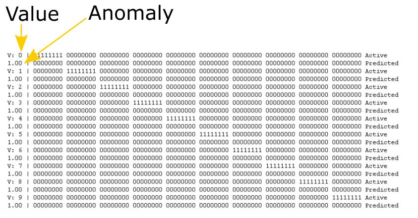
As expected, there are two rows per encoded number (active/actual bits and the predicted bits).
The first column of the line with the active bits shows the actual integer value, the anomaly is displayed on the line with the predicted bits. 1.00 means 100%.

The algorithm doesn’t predict anything yet, hence the anomaly is always 100%. That is because it has never seen any of the encoded values before and therefore it is not trying to predict anything.

So let’s change that and add a second cycle.

Predicting

import numpy as np
from htm.bindings.sdr import SDR
from htm.algorithms import TemporalMemory as TM

def formatSdr(sdr):
  result = ''
  for i in range(sdr.size):
    if i > 0 and i % 8 == 0:
      result += ' '
    result += str(sdr.dense.flatten()[i])
  return result

arraySize = 80
cycleArray = np.arange(0, 10, 1)
inputSDR = SDR( arraySize )

tm = TM(columnDimensions = (inputSDR.size,),
        cellsPerColumn=1,       # default: 32
        minThreshold=4,         # default: 10
        activationThreshold=8,  # default: 13
        initialPermanence=0.5,  # default: 0.21
        )

for cycle in range(2):
    for sensorValue in cycleArray:
        sensorValueBits = inputSDR.dense
        sensorValueBits = np.zeros(arraySize)
        sensorValueBits[sensorValue * 8:sensorValue * 8 + 8] = 1
        inputSDR.dense = sensorValueBits

        tm.compute(inputSDR, learn = True)
        print(format(sensorValue,'>2') + '/' + format(cycle, '1d')+ ' |', formatSdr(tm.getActiveCells()), 'Active')
    
        tm.activateDendrites(True)
        print(format(tm.anomaly, '.2f') + ' |', formatSdr(tm.getPredictiveCells()), 'Predicted')

I’ve essentially just added line 24, to get two cycles of the iteration from 0 to 9 now. The cycle number is added to the print statement in line 32.

What do we get this time?

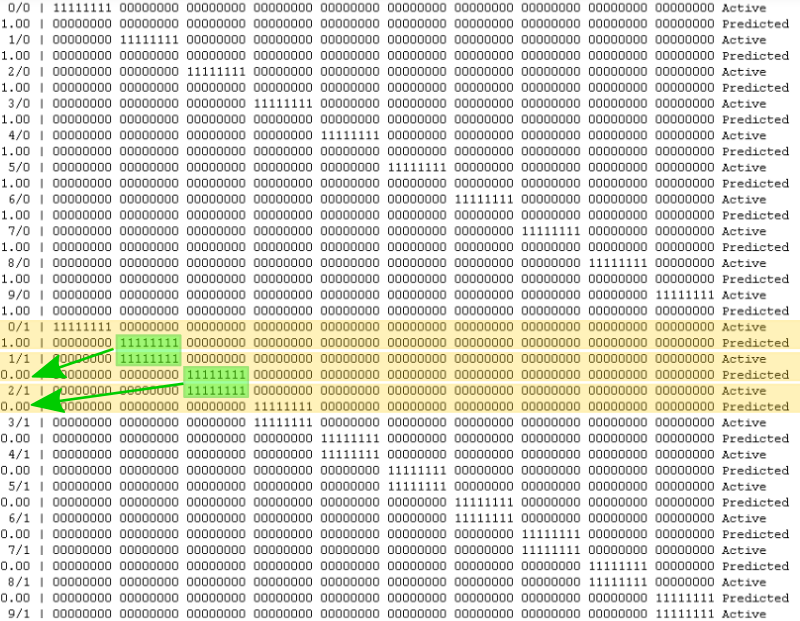
Excellent. Prediction starts from the line beginning with 0/1. And in the next step (1/1) we can see that the predicted encoding actually matches. This is also reflected in the value returned by tm.anomaly.

Epilogue

Congratulations on getting this far. I know that’s a lot of information to digest.

Now, however, we have acquired some fundamental knowledge with which we can dive more into htm.core, soon.

So stay tuned for the next part, which will continue where that part left off